Use PCA to determine if useful synthetic dimensions exist.
PCA interpretation and plotting
Scott Gabara
12/12/2016
PCA
#PCA
str(iris)
## 'data.frame': 150 obs. of 5 variables:
## $ Sepal.Length: num 5.1 4.9 4.7 4.6 5 5.4 4.6 5 4.4 4.9 ...
## $ Sepal.Width : num 3.5 3 3.2 3.1 3.6 3.9 3.4 3.4 2.9 3.1 ...
## $ Petal.Length: num 1.4 1.4 1.3 1.5 1.4 1.7 1.4 1.5 1.4 1.5 ...
## $ Petal.Width : num 0.2 0.2 0.2 0.2 0.2 0.4 0.3 0.2 0.2 0.1 ...
## $ Species : Factor w/ 3 levels "setosa","versicolor",..: 1 1 1 1 1 1 1 1 1 1 ...head(iris)## Sepal.Length Sepal.Width Petal.Length Petal.Width Species
## 1 5.1 3.5 1.4 0.2 setosa
## 2 4.9 3.0 1.4 0.2 setosa
## 3 4.7 3.2 1.3 0.2 setosa
## 4 4.6 3.1 1.5 0.2 setosa
## 5 5.0 3.6 1.4 0.2 setosa
## 6 5.4 3.9 1.7 0.4 setosa# apply PCA - scale. = TRUE is highly advisable, but default is FALSE
iris.spp <- iris[, 5] # set species column 5 to use later
iris.pca <- prcomp(iris[,1:4],
center = TRUE,
scale. = TRUE)
par(mfrow=c(1,2))
print(iris.pca)## Standard deviations:
## [1] 1.7083611 0.9560494 0.3830886 0.1439265
##
## Rotation:
## PC1 PC2 PC3 PC4
## Sepal.Length 0.5210659 -0.37741762 0.7195664 0.2612863
## Sepal.Width -0.2693474 -0.92329566 -0.2443818 -0.1235096
## Petal.Length 0.5804131 -0.02449161 -0.1421264 -0.8014492
## Petal.Width 0.5648565 -0.06694199 -0.6342727 0.5235971plot(iris.pca, type = "l") # scree plot for inspecting variance, adds to the number of variables, in this case 4.
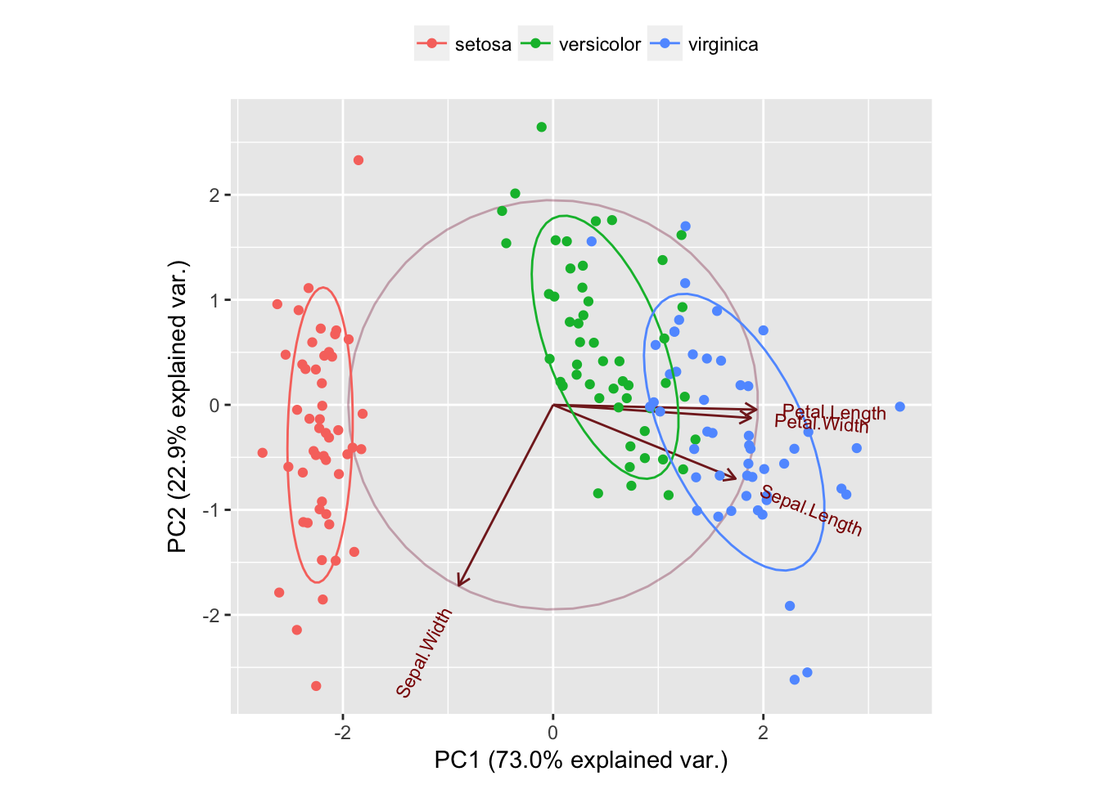
summary(iris.pca) # PCs are the number of variables and sum to that number, in this case 4. The synthetic dimension PC 1 explains 0.7296 (72.96%) of the variation in observations.## Importance of components:
## PC1 PC2 PC3 PC4
## Standard deviation 1.7084 0.9560 0.38309 0.14393
## Proportion of Variance 0.7296 0.2285 0.03669 0.00518
## Cumulative Proportion 0.7296 0.9581 0.99482 1.00000predict(iris.pca, newdata=tail(iris[,1:4], 2))## PC1 PC2 PC3 PC4
## 149 1.3682042 -1.00787793 -0.9302787 0.02604141
## 150 0.9574485 0.02425043 -0.5264850 -0.16253353biplot(iris.pca) # Visualize PCA
# ggplot version
#library(devtools)
library(ggbiplot)
g2 <- ggbiplot(iris.pca, obs.scale = 1, var.scale = 1, groups = iris.spp, ellipse = TRUE, circle = TRUE)
g2 <- g2 + scale_color_discrete(name = '')
g2 <- g2 + theme(legend.direction = 'horizontal', legend.position = 'top')
g2
#library(devtools)
library(ggbiplot)
g2 <- ggbiplot(iris.pca, obs.scale = 1, var.scale = 1, groups = iris.spp, ellipse = TRUE, circle = TRUE)
g2 <- g2 + scale_color_discrete(name = '')
g2 <- g2 + theme(legend.direction = 'horizontal', legend.position = 'top')
g2